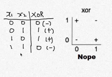
XOR에 대한 내용이다.
x1, x2이 서로 같은 값이면 0, 다른값이면 1을 갖는다.
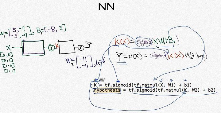
XOR 문제를 Neural network로 풀어보자
w,b를 추가로 만들어 layer를 생성하고 그 layer를 다른 layer에 씌우는 과정이다.
이 과정이 많아질수록 정확도가 높아진다.
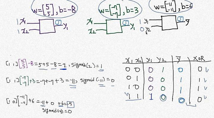
위 과정은 x1, x2를 (w1,b1), (w2,b2)의 layer 를 통해서 y1,y2를 만들고 (w3,b3)으로 y를 출력하여 XOR값과 일치하는지 확인하는 내용이다.
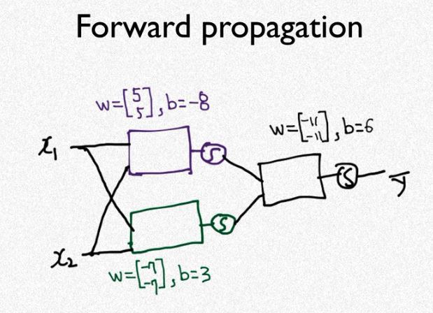
위 과정을 간략하게 나타내면 위의 전개도와 같다.
# Lab 9 XOR
import tensorflow as tf
import numpy as np
tf.set_random_seed(777) # for reproducibility
learning_rate = 0.1
x_data = [[0, 0],
[0, 1],
[1, 0],
[1, 1]]
y_data = [[0],
[1],
[1],
[0]]
x_data = np.array(x_data, dtype=np.float32)
y_data = np.array(y_data, dtype=np.float32)
X = tf.placeholder(tf.float32, [None, 2])
Y = tf.placeholder(tf.float32, [None, 1])
#neural network의 layer1
W1 = tf.Variable(tf.random_normal([2, 2]), name='weight1')
b1 = tf.Variable(tf.random_normal([2]), name='bias1')
layer1 = tf.sigmoid(tf.matmul(X, W1) + b1)
#neural network의 layer2
W2 = tf.Variable(tf.random_normal([2, 1]), name='weight2')
b2 = tf.Variable(tf.random_normal([1]), name='bias2')
hypothesis = tf.sigmoid(tf.matmul(layer1, W2) + b2)
# cost/loss function
cost = -tf.reduce_mean(Y * tf.log(hypothesis) + (1 - Y) *
tf.log(1 - hypothesis))
train = tf.train.GradientDescentOptimizer(learning_rate=1e-1).minimize(cost)
# Accuracy computation
# True if hypothesis>0.5 else False
predicted = tf.cast(hypothesis > 0.5, dtype=tf.float32)
accuracy = tf.reduce_mean(tf.cast(tf.equal(predicted, Y), dtype=tf.float32))
# Launch graph
with tf.Session() as sess:
# Initialize TensorFlow variables
sess.run(tf.global_variables_initializer())
for step in range(5001):
sess.run(train, feed_dict={X: x_data, Y: y_data})
if step % 100 == 0:
print(step, sess.run(cost, feed_dict={
X: x_data, Y: y_data}), sess.run([W1, W2]))
# Accuracy report
h, c, a = sess.run([hypothesis, predicted, accuracy],
feed_dict={X: x_data, Y: y_data})
print("\nHypothesis: ", h, "\nCorrect: ", c, "\nAccuracy: ", a)
#layer를 추가한 문장 이외의 나머지 부분은 logistic regression 소스와 같다.
#layer만 추가했기 때문에 neural network을 적용, 미적용한 코드를 비교해보도록 하겠다.
* neural network 비교
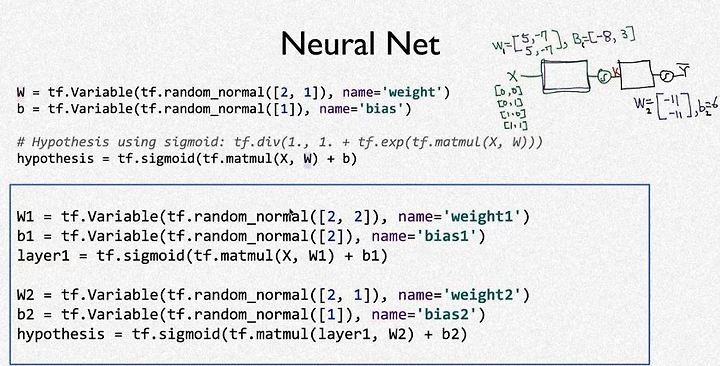
위 그림에서 파란색 박스친곳의 내용이 neural network(NN)의 구성이다.
박스 위는 일반적인 XOR의 구성이다.
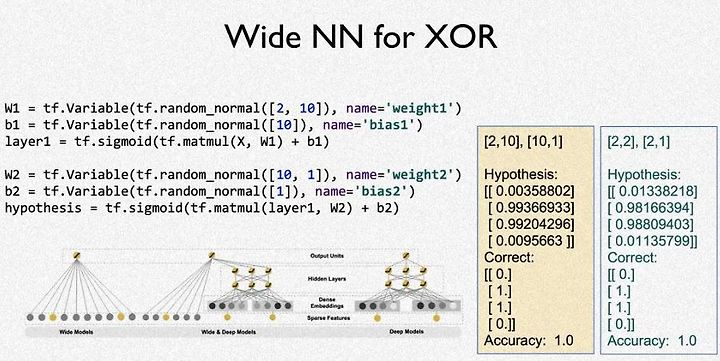
사용자에 따라서 NN을 여러가지 방법으로 구현할 수 있다.
위 그림은 wide NN인데 [2,2]행렬의 값을 -> [2,10] -> [10,1] 출력 하는 방법이다.
일반적인 NN보다 약간 더 정확도가 높은것을 볼 수 있다(오른쪽 그림의 hypothesis)
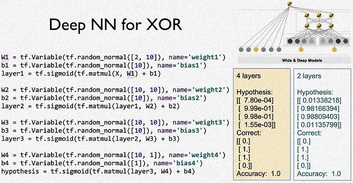
Deep NN이라고 소개 되어진다.
layer를 무수히 많이 쌓는 방법이다.
layer를 어떻게 쌓느냐에 따라 정확도가 달라지겠지만 아직 예제에 나온 수준에서 건드리는게 내가 할 수 있는 최대한의 접근인것 같다.
위 방법은
[2,2] -> [2,10] -> [10,10] -> [10,10] -> [10,1] 와 같이 전개되어진다.
앞에 소개된 wide NN보다 더 정확한 것을 볼 수 있다.